DDGI Dev Notes
This post documents a basic implementation of DDGI based on the 2019 paper1. Implementation accounts for only the diffuse components.
Ray-Queried Light Visibility
By leveraging Vulkan’s acceleration structures and ray query shader functions, I can get a clean representation of light visibility from any point in the scene. First, build an acceleration structure out of the scene. The table below shows mapping between glTF concepts, engine objects, and Vulkan acceleration structures
| glTF | My Engine | BLAS | TLAS |
| mesh | renderable | geometry | – |
| node | scene node | BLAS | instance |
| scene | scene | – | TLAS |
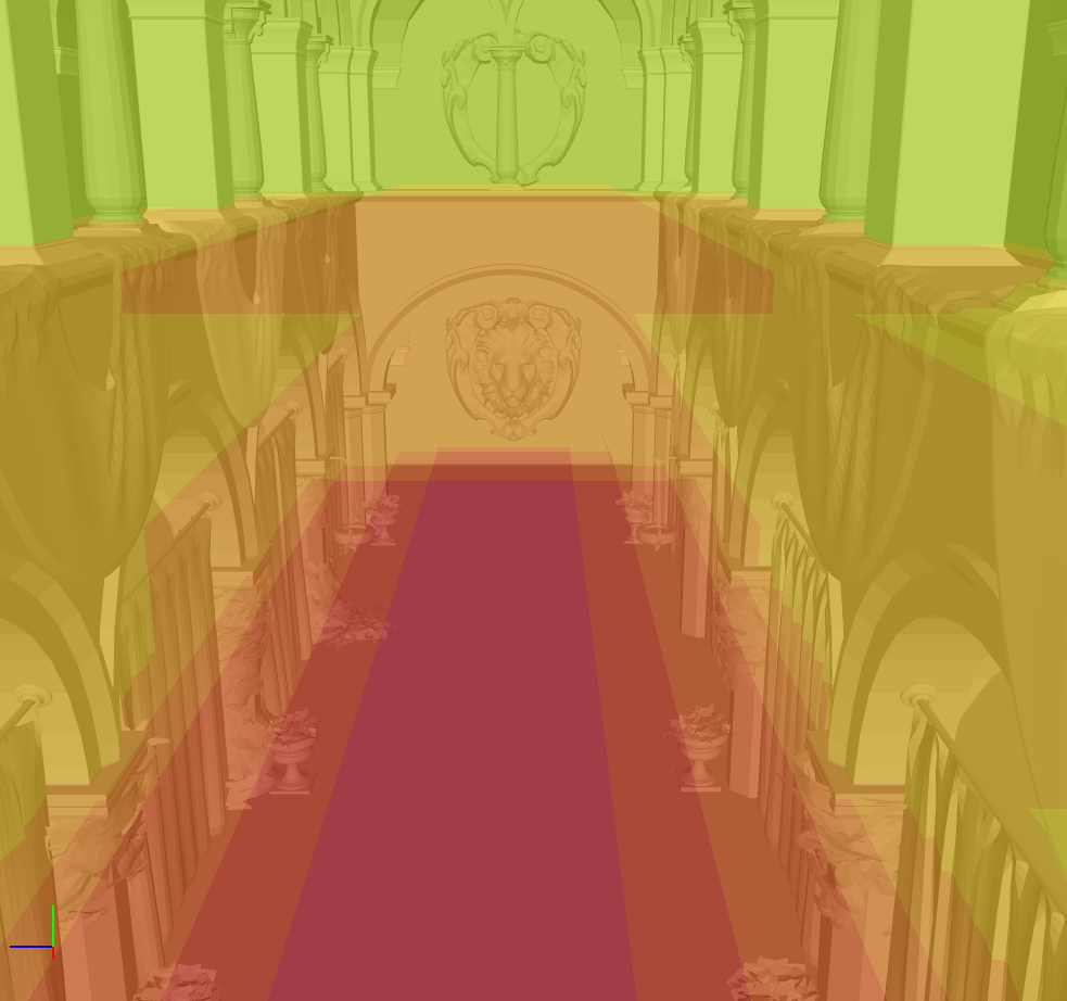
Image on the left shows AABB overlap. Image on the right is a traversal timing heatmap. Both views are captured with NSight Graphics.
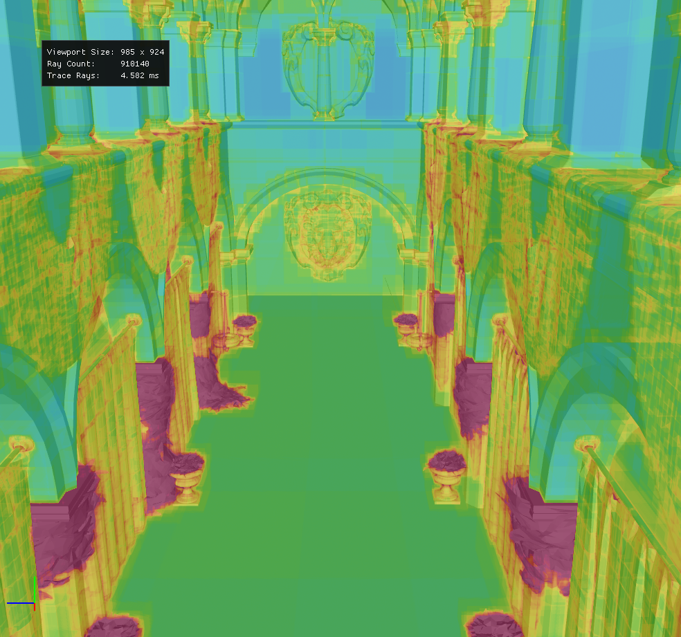
Non-opaque primitives, in this case alpha masked foliage, are the most expensive to traverse because intersections with them are often not committed. Traversal must continue through multiple non-opaque intersections until the ray hits a nearby opaque wall.
Another problem is poor AABB geometry grouping. The flowerpots, pillars, and curtains on the lower level are grouped into large meshes whose parts share the same materials. These meshes contain large empty spaces. Their AABBs therefore overlap significantly, making the BLAS less compact and less efficient to traverse.
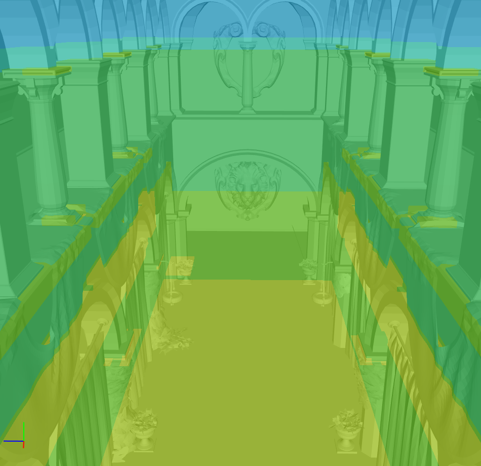
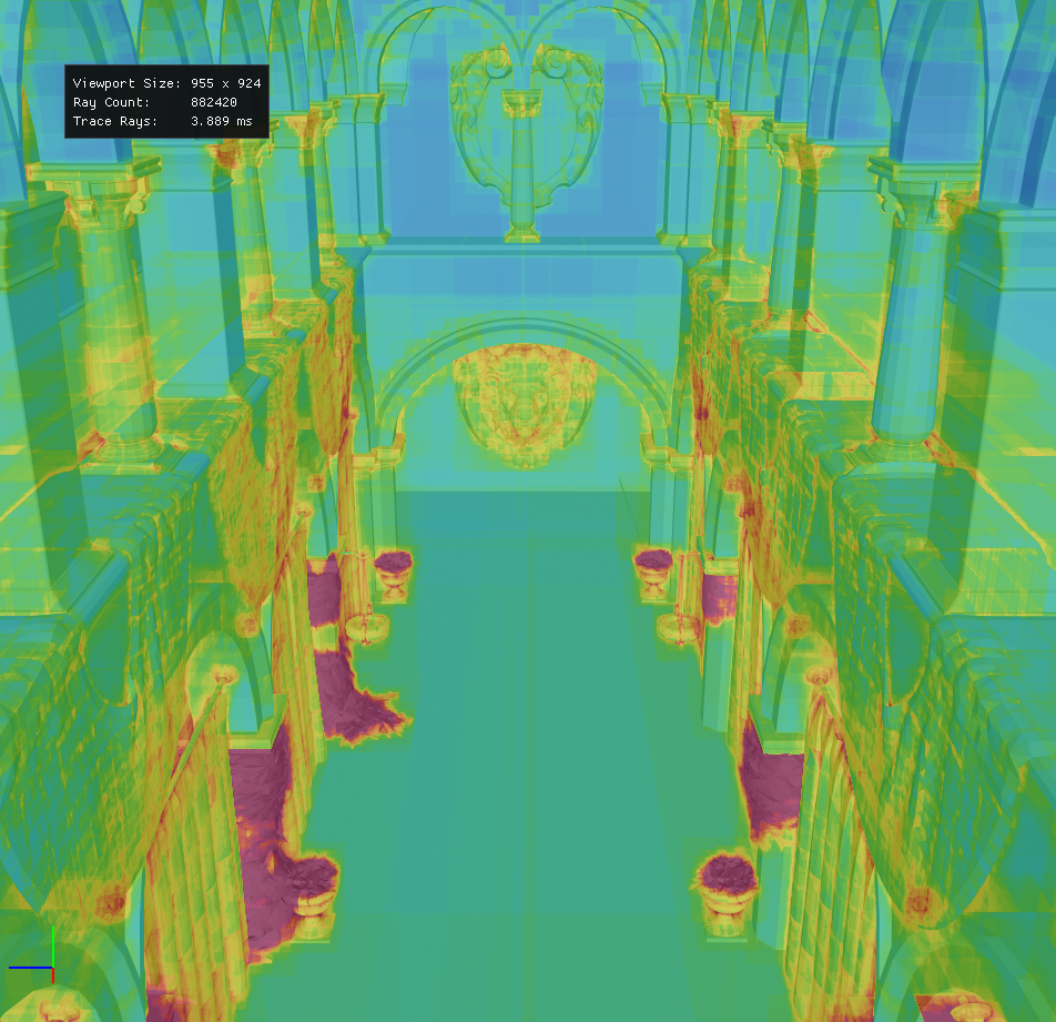
The solution is simple: separate the meshes. The image on the left shows less AABB overlap, while the image on the right shows faster traversal, if you look hard enough. Nsight measurements from the same viewpoint show that the ray tracing time dropped from 4.5 ms to 3.8 ms.
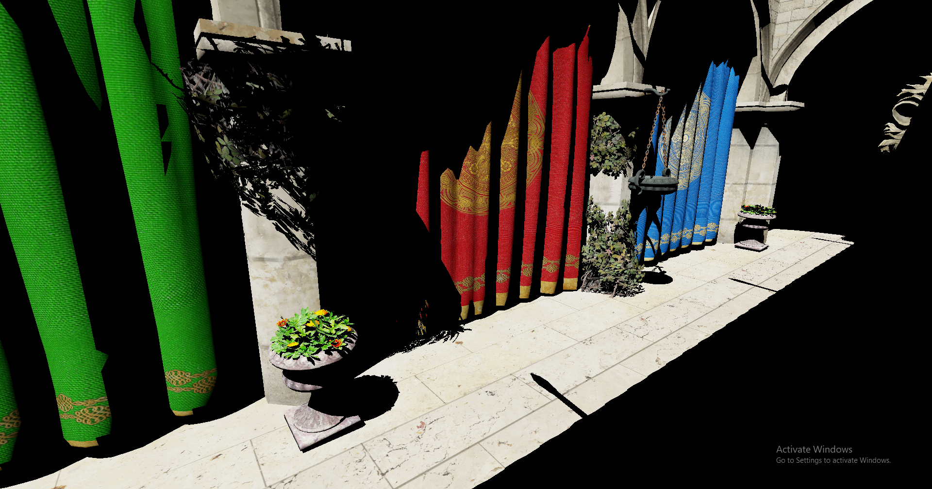
The image below was generated by tracing rays from the camera in the direction of each screen pixel. Only direct lighting with a Lambertian diffuse BRDF is accounted for. This is often enough for indirect lighting unless you’re aiming for sharp caustics reflected off metallic surfaces.
Notice the pixel perfect shadows, which is a signature visual cue of ray queries. Also notice the heavy moire patterns caused by the lack of mipmapping. Since I’ll be averaging the radiance later in the process, these artifacts won’t matter.
By changing the ray origins from the camera to each probe’s location, and replacing screen pixels with samples on a sphere, the same ray query architecture can be used to sample radiance from probes at arbitrary points in space.
In this example, I placed a 16 × 8 × 16 grid of probes throughout the Sponza scene and traced 192 rays from each probe. The four textures generated from a single tracing pass contains the hit points’ direct radiance, positions, normals, albedo, and metallic-roughness values, as shown below.





Probe Placement in Blender
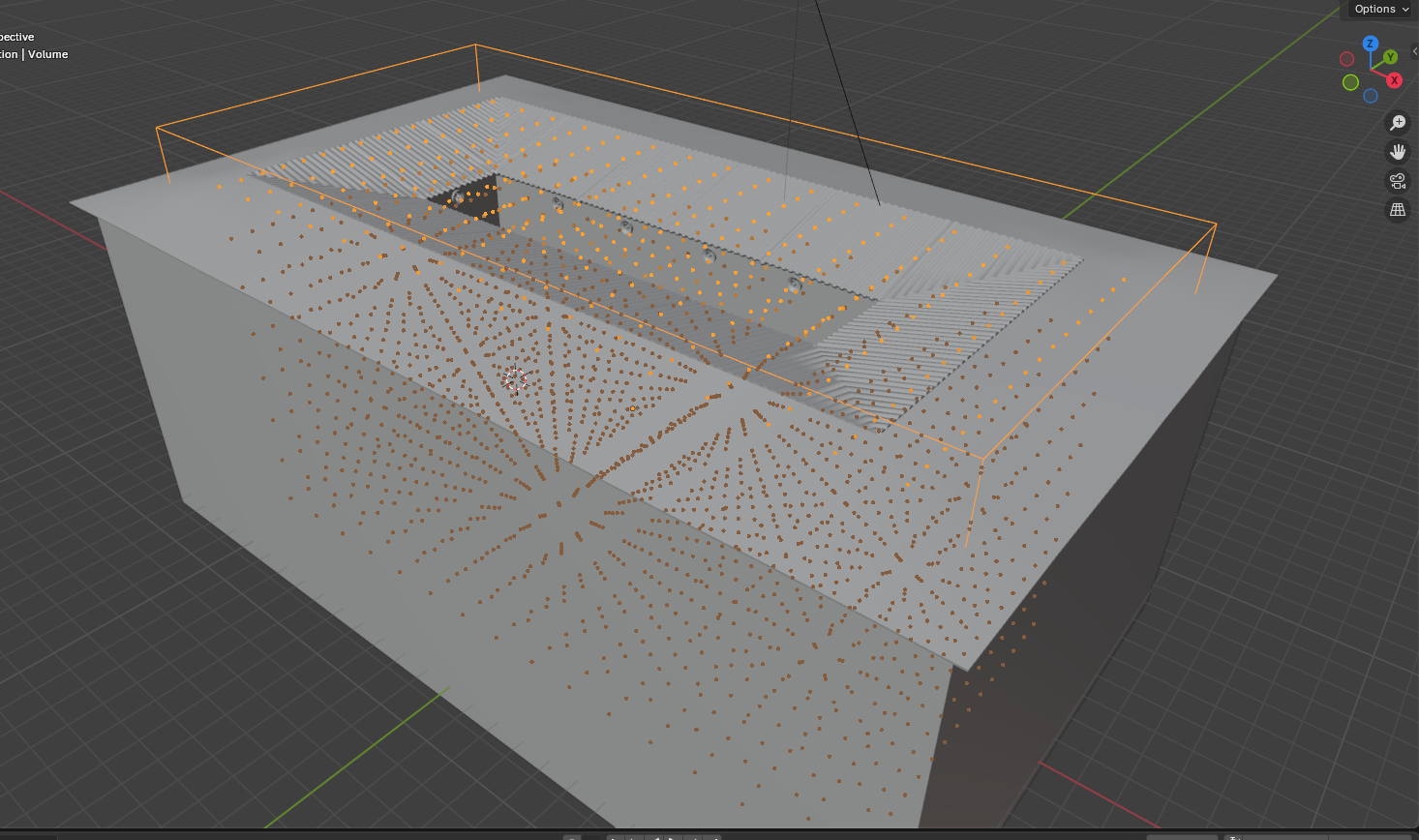
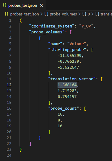
A proper editor is out of the scope of my current work. So I took it to Blender to author probe fields for my renderer. Since DDGI inherently prevents light leaking regardless of probe placement, I only needed to create an axis-aligned probe field and export its corner position, along with the constant spacing between neighboring probes. This was done by running a small script inside Blender.
Probe Data Atlas
The original DDGI paper divides probe update into multiple substeps including depth filtering, actual probe data update and copying edges. Since Vulkan is so versatile, my probe update is done in a single compute pass with in-shader barriers to synchronize probe data and edge data writes.
Irradiance
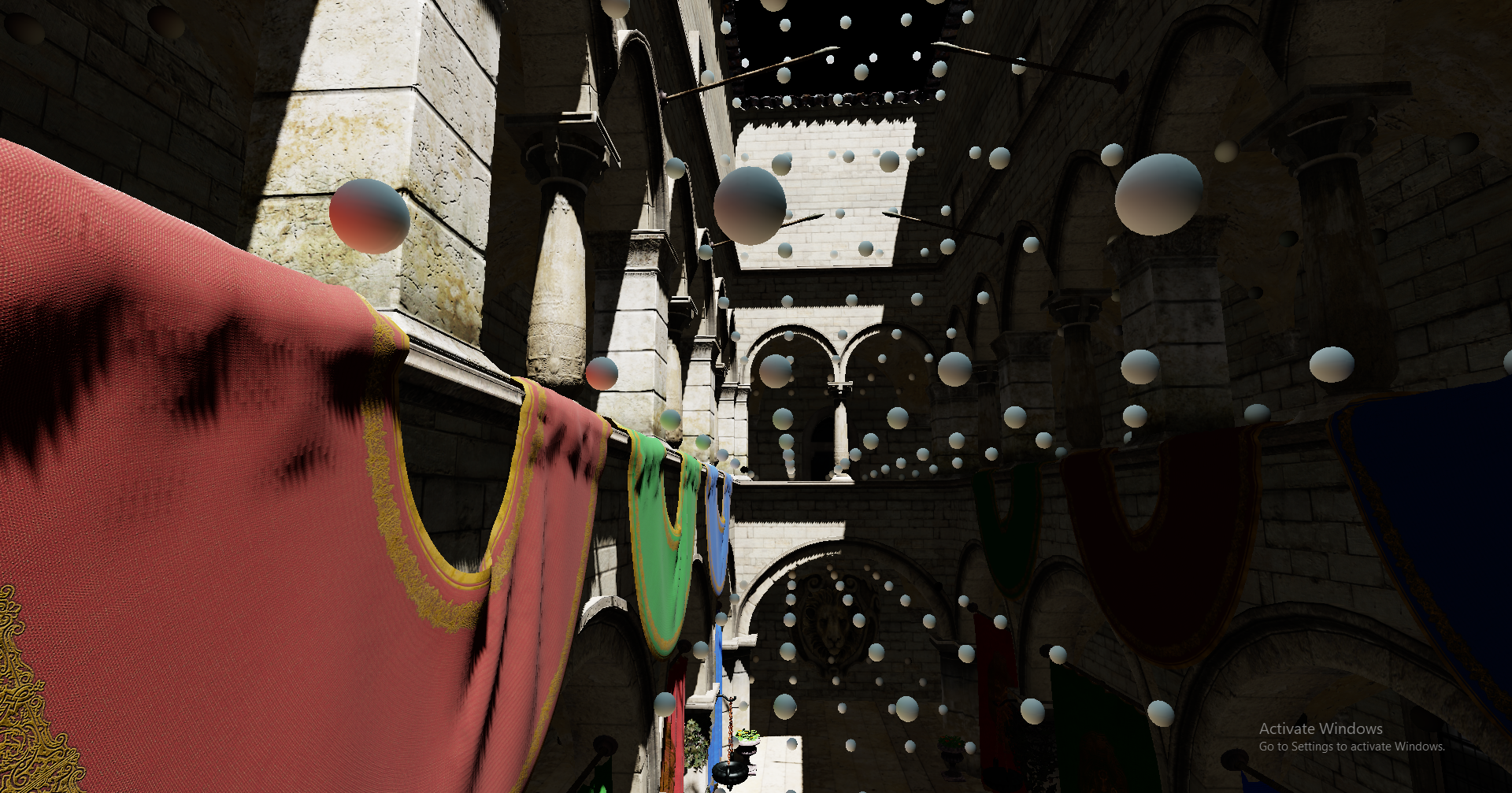
Should be more rigorously called the cosine-weighted average radiance. Borders are added to each probe to accommodate linear sampling across octahedral encoding’s seams. Observe layers of probes from ground level all the way to the roof.

Depth
Depth atlas encodes weighted average of occluder distance and weighted average of squared occluder distance in R and G channels respectively. That is the reason why the atlas appears to be yellow. Darker regions indicate the presence of occluders.

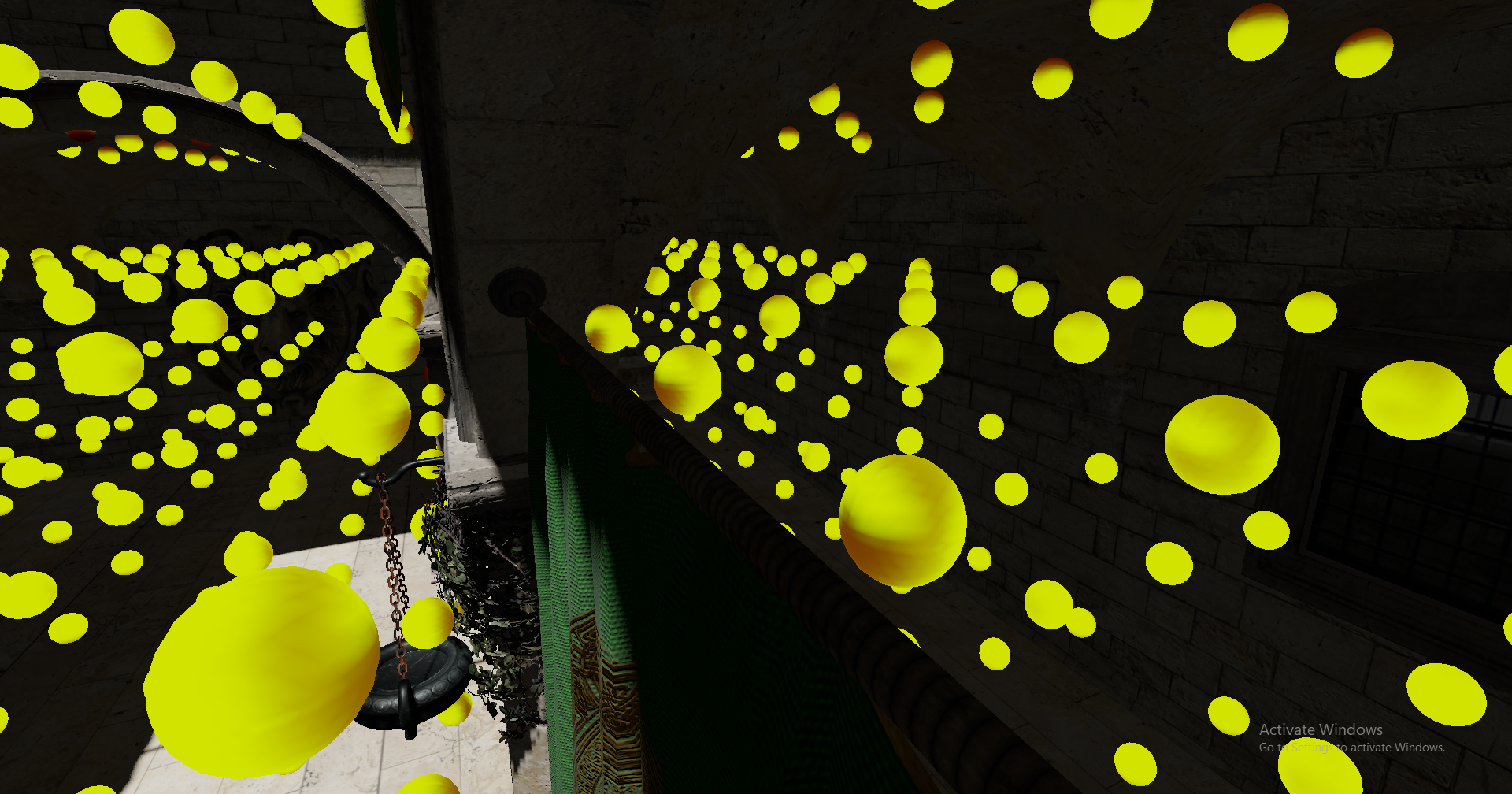
Irradiance Probes Debug Draw
Depth Probes Debug Draw
Temporal Denoising
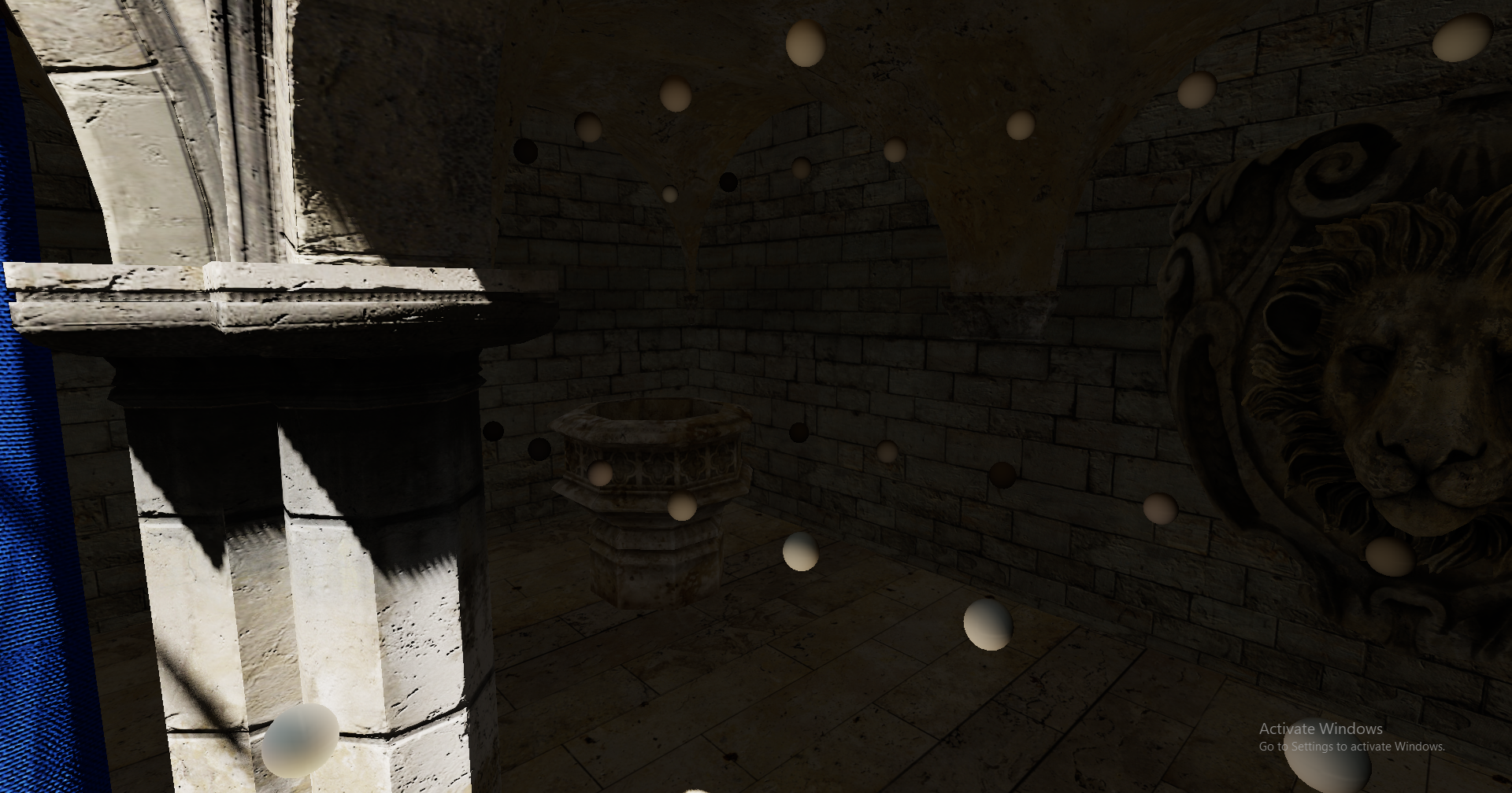
Without temporal denoising, probes in well-lit regions capture their surroundings reasonably well. However, probes in darker regions that receive only a small amount of light produce wildly unreliable results. The image below illustrates this problem. Notice how bright and dim probes alternate near the corner.
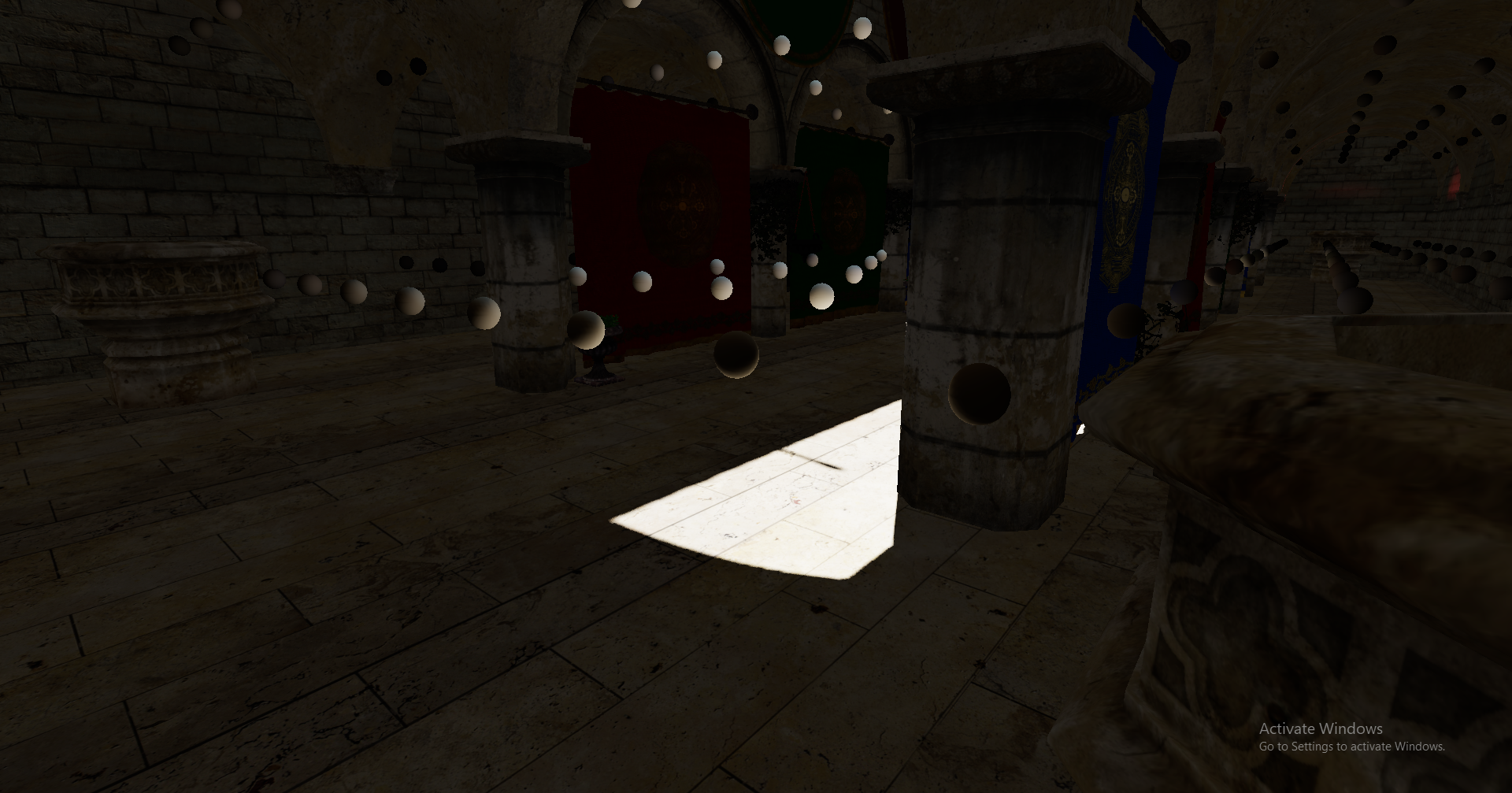
The image below shows the small patch of light visible to probes tucked away in the same corner. If you plotted the radiance distribution across one of these probes’ spherical surfaces, this patch would appear as a sharp spike. Discrete samples on a spherical surface, in this case, generated using a spherical Fibonacci sequence, can sometimes miss such high-frequency spatial variations.
Drastically increasing the sample count to 1,024 or even 2,048 rays per probe per frame could mitigate this effect, but it would completely tank performance. Instead, I rotate the Fibonacci sequence every frame, then blend the current frame’s atlas with the previous frame’s. This distributes the samples across multiple frames while keeping the workload per frame low. This is how temporal denoising works during probe updates.
Temporal denoising requires some fine tuning. The authors refer to the blend weight of the history atlas as ‘hysteresis’. If the hysteresis is too high, the probes become less responsive to changes in the scene, creating a lingering effect. If it is too low, flickering becomes more pronounced.
This method prompted me to add support for history resources to my frame graph implementation. See the OTCV repository for details. Here is the result after temporal denoising:
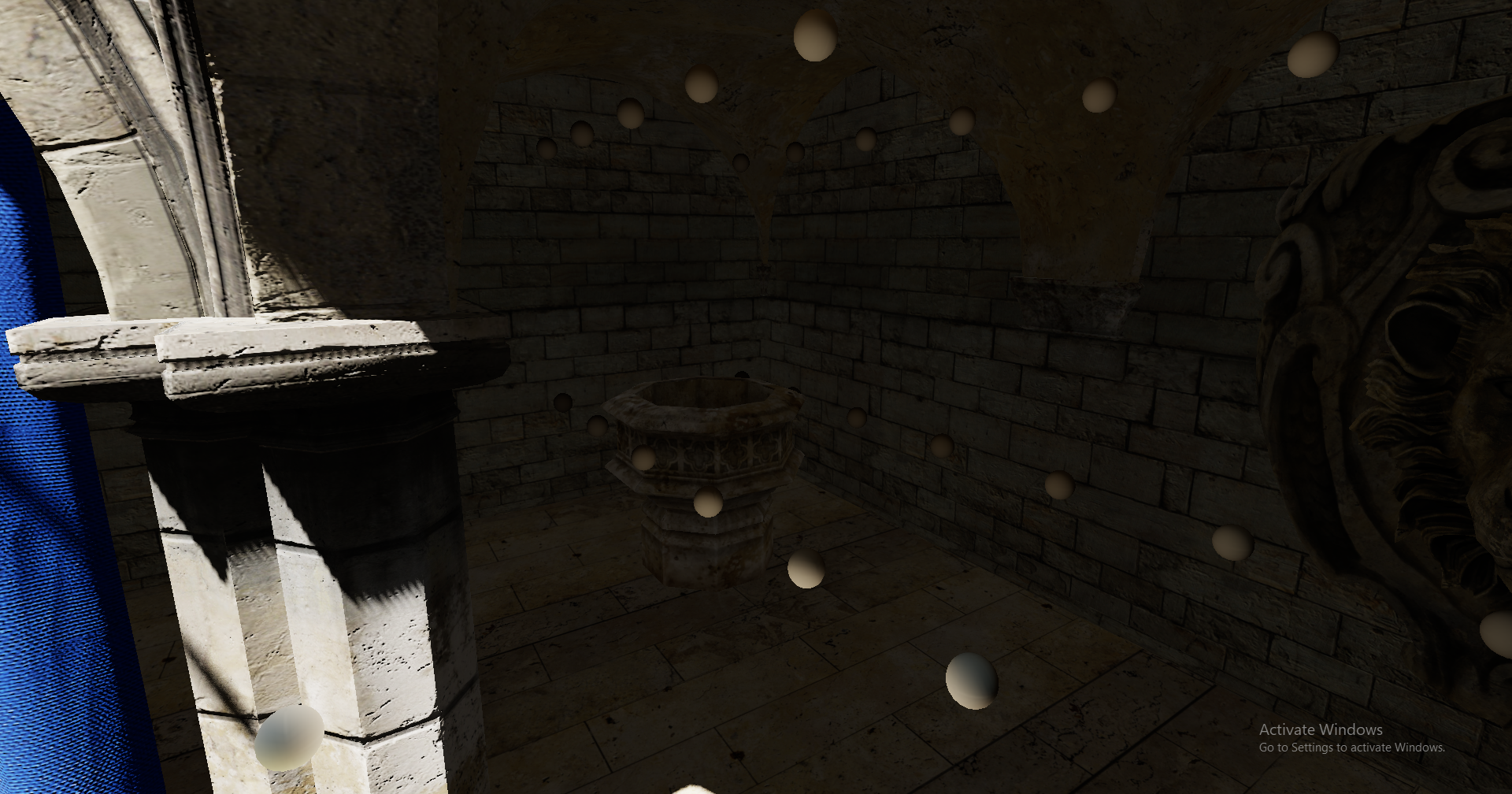
Good. No more alternating dim and bright probes.
A similar idea also appears in rigid-body collision resolution, where warm starting carries cached impulses across frames. This allows the solver to reuse previous results instead of starting from scratch every frame.
Multi-Bounce
At first, I thought single-bounce indirect lighting was visually convincing enough. However, while adding skylight to the Sponza scene, I realized that it could not reach regions without a direct line of sight to the sky. Only through multiple bounces can skylight find its way into every corner of the scene.
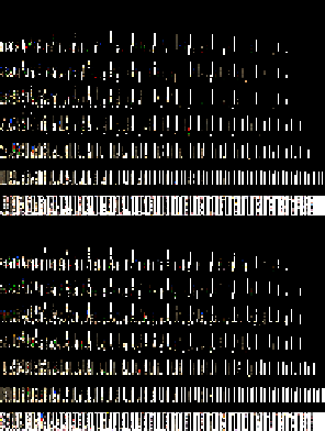
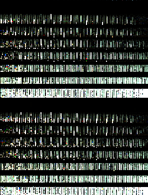
Multi-bounce lighting is easily achieved by adding a probe sampling pass and additively blending its output with the existing direct-lighting query results. Left shows a snippet of direct light radiance captured. Right shows the same snippet with indirect radiance from previous frame blended in
With this approach, I can in theory recreate the scene demonstrated by the DDGI authors, where an entire bathroom is illuminated using only skylight.
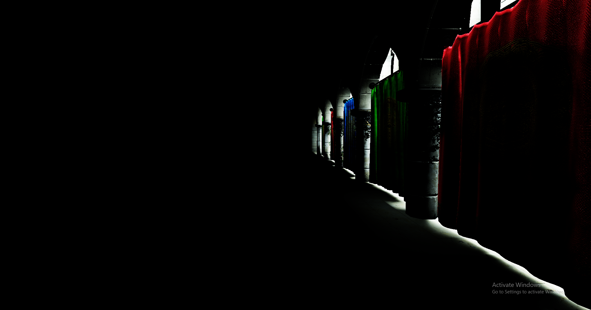
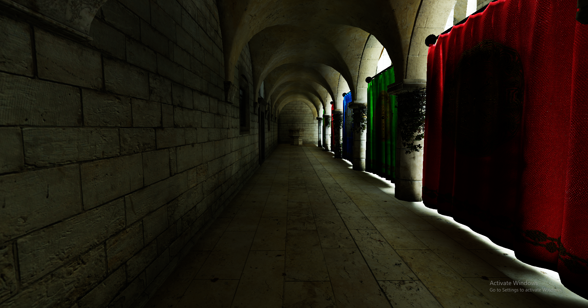
Below is a comparison between single-bounce and multi-bounce lighting. Neither case uses direct lighting. The back of the curtain is supposed to be illuminated by light bouncing off surfaces in the atrium on the other side.
Putting It All Together
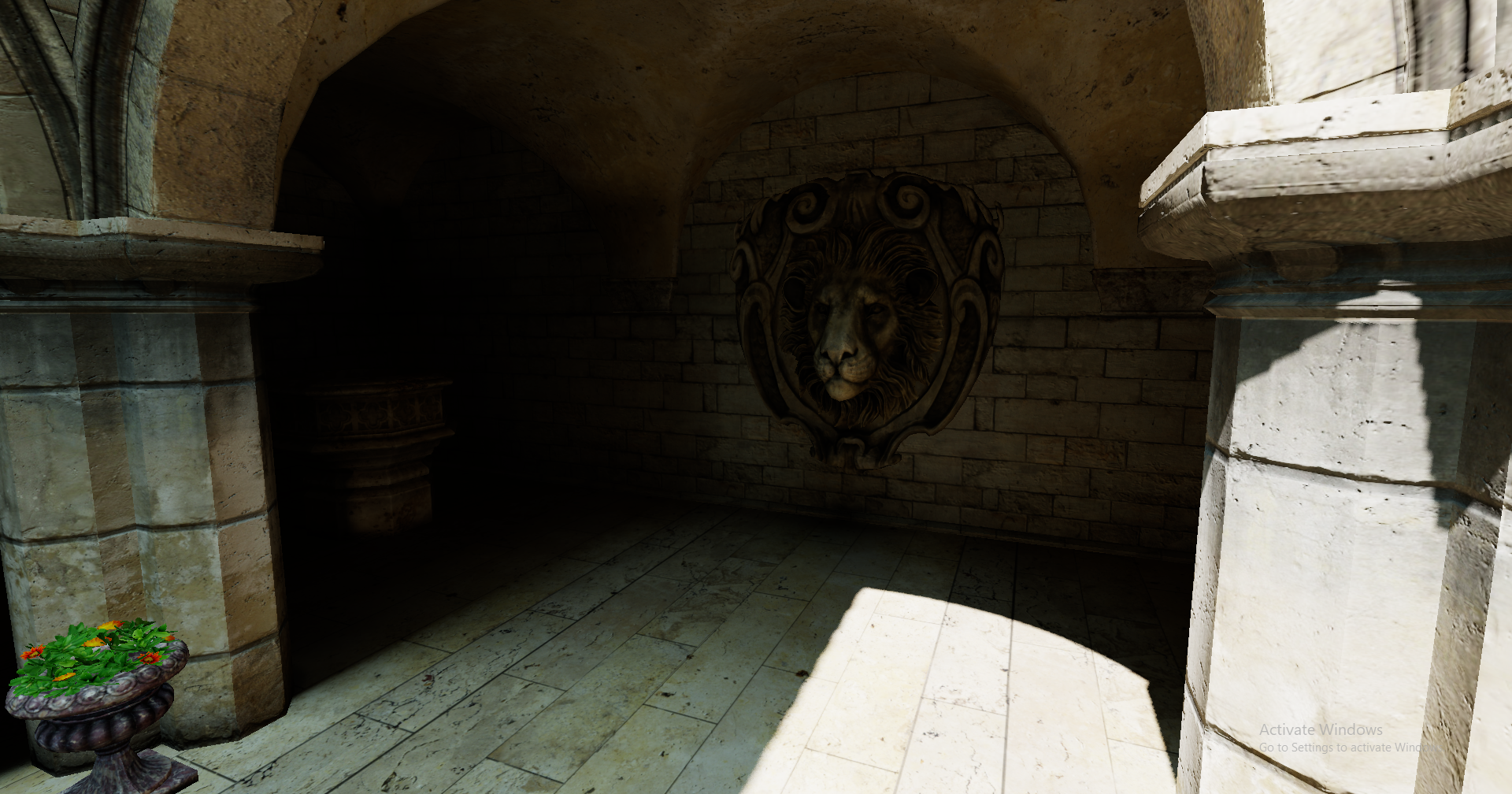
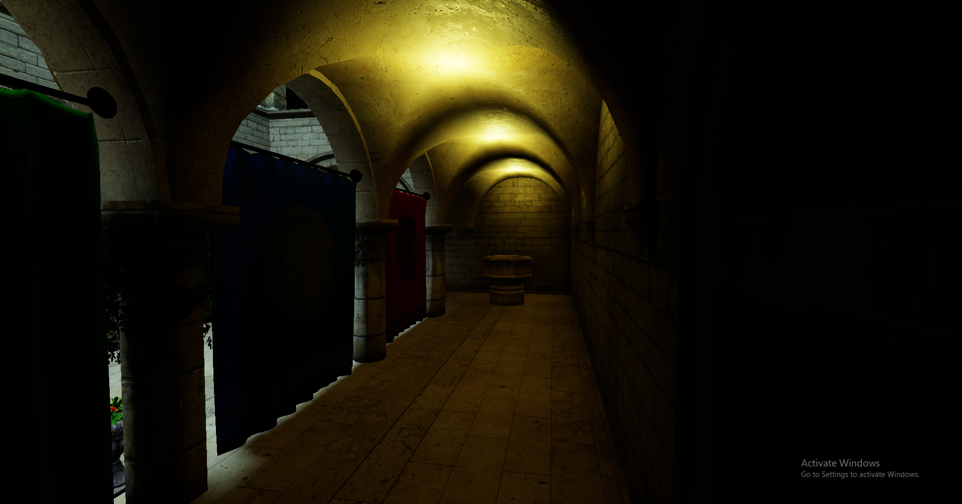
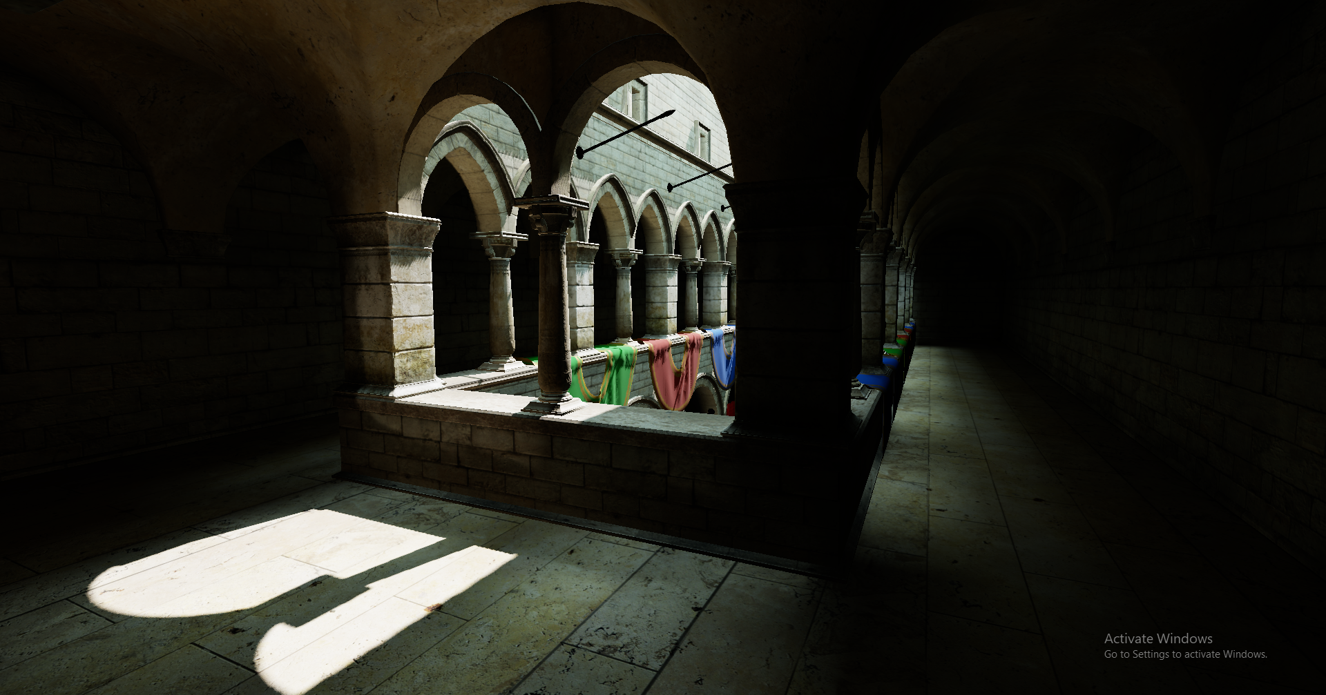
Every point light in the second image is set to have a very limited influence radius. They can only directly light up the arch roof above them. That is the reason why the basin in the far corner does not cast a defined shadow. Indirect lighting alone creates this dim and soft aesthetic like a wine cellar.
Caveats and Possible Improvements
- Light culling and clustering problem. Every ray query needs to know which light affects the point where the ray hits. My existing light culling and clustering system only works in view space. Since probes are scattered across the entire scene, there is no universal view space for all of the probes. So I iterated through all lights. That is going to be problematic performance-wise if light count gets really high. Consider world space light culling. Create a scene-wide grid and rasterize light influence sphere within this grid. Both view space light clustering and ray query light clustering could be incorporated into this architecture.
- Probe update frequence. Probes far away from camera or placed near static objects could update at a much lower rate.
- Area light or emissive material handling.
- Reflective probes