Fitting Parameters for the Linearly Transformed Cosine
This blog post explains the thoughts and implmentation details behind the fitting of Linearly Transformed Cosine (LTC) parameters to GGX BRDF. Largely inspired by Eric Heitz’s LTC research1. Paramter normalization caveats discussed in Stephen Hill’s lecture on the implementation details2 are also accounted for.
Parameterization
The objective is to construct a transformation $\mathbf{M}$ that, when applied to the hemispherical cosine distribution, is designed to approximate the GGX BRDF as closely as possible. To this end, multiple textures are employed to store tabulated parameters representing $\mathbf{M}$, indexed by pairs of roughness $\sqrt{\alpha}$ and viewing angle $\theta_v$, which span the $u$ and $v$ directions of texture space, respectively.
\[\mathbf{M} = \mathbf{B}\mathbf{m}\]$\mathbf{m}$ is a transformation that scales the cosine lobe in $x$ and $y$ direction, in the meantime shearing $x$ with respect to $z$. $\mathbf{m}$ does not skew $y$, effectively keeps the transformed distribution symmtric with respect to the $xOz$ plane. Jacobian of this transformation will ensure $z$ component being scaled accordingly to keep the transformed distribution normalized.
\[\begin{equation} \mathbf{m} = \begin{bmatrix} m_{11} & 0 & m_{13} \\ 0 & m_{22} & 0 \\ 0 & 0 & 1 \end{bmatrix} \label{eq:m-x-shear} \end{equation}\]The $\mathbf{m}$ in Eric Heitz’s implementation also includes a non-zero $y$-shearing parameter $m_{23}$, raising the optimization dimensions to four. After the optimization process completes, $m_{23}$ is usually found to be negligible and is simply ignored. We find that introducing $m_{23}$ is redundant and therefore settle on only three optimization dimensions.
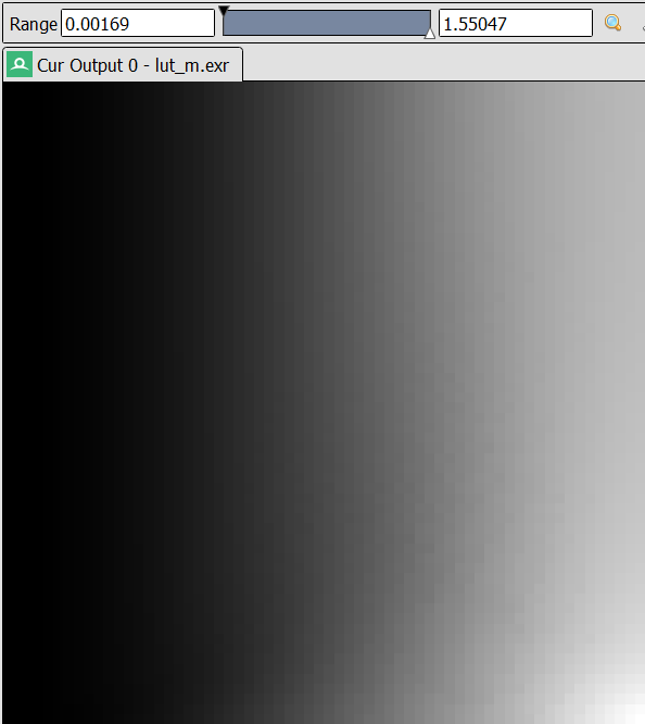
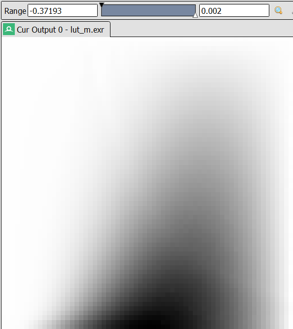
Tabulated parameters of $\mathbf{m}$ are listed in Figure 1.

$\mathbf{B}$ is a rotation matrix around the $+y$ axis:
\[\mathbf{B} = \begin{bmatrix} \cos\bar{\theta_i} & 0 & -\sin\bar{\theta_i} \\ 0 & 1 & 0 \\ \sin\bar{\theta_i} & 0 & \cos\bar{\theta_i} \end{bmatrix}\]$\bar{\theta_i}$ is the polar angle of weighted average incident direction $\bar{\omega_i}$ given an outgoing direction $\omega_o$:
\[\bar{\omega_i} = \int_{\Omega} f_r(\omega_i, \omega_o)\cos\theta_i\omega_id\omega_i\]Notice the similarity between the above weighted average and the definition of albedo:
\[Albedo = \int_{\Omega} f_r(\omega_i, \omega_o)\cos\theta_id\omega_i\]Since $\bar{\omega_i}$ is typically computed from a known BRDF (in our case, GGX), only the three scaling and shearing parameters of the matrix $\mathbf{m}$ require fitting. This separation of rotation from shearing-scaling factors, as opposed to directly fitting all five parameters of $\mathbf{M}$, reduces the likelihood of converging to a local minimum. Consequently, it yields more consistent results across adjacent entries in the resulting LUTs.
Expanded form of $\mathbf{M}$:
\[\mathbf{M} = \begin{bmatrix} m_{11}\cos\bar{\theta_i} & 0 & m_{13}\cos\bar{\theta_i}-\sin\bar{\theta_i} \\ 0 & m_{22} & 0 \\ m_{11}\sin\bar{\theta_i} & 0 & m_{13}\sin\bar{\theta_i}+\cos\bar{\theta_i} \end{bmatrix} = \begin{bmatrix} a & 0 & b \\ 0 & c & 0 \\ d & 0 & e \end{bmatrix}\]The LTC paper divides $\mathbf{M}$ by its bottom right component $e$ to save one tabulated parameter. But in practice it is seen as a “false economy”2 because a second texture storing albedo has to be introduced regardless. We compute and tabulate this “normalized” matrix only to compare against the results given by Eric Heitz in his original paper. The normalized $\mathbf{\hat{M}}$:
\[\mathbf{\hat{M}} = \frac{1}{e}\mathbf{M} = \begin{bmatrix} \dfrac{a}{e} & 0 & \dfrac{b}{e} \\[8pt] 0 & \dfrac{c}{e} & 0 \\[8pt] \dfrac{d}{e} & 0 & 1 \\[8pt] \end{bmatrix} = \begin{bmatrix} \hat{a} & 0 & \hat{b} \\[8pt] 0 & \hat{c} & 0 \\[8pt] \hat{d} & 0 & 1 \\[8pt] \end{bmatrix}\]It is also convenient to write paramters of $\mathbf{M^{-1}}$ and $\mathbf{\hat{M}^{-1}}$ to an LUT for later use in real-time polygonal lighting.
\[\mathbf{M^{-1}} = \begin{bmatrix} \dfrac{e}{\Delta} & 0 & -\dfrac{b}{\Delta} \\[8pt] 0 & \dfrac{1}{c} & 0 \\[8pt] -\dfrac{d}{\Delta} & 0 & \dfrac{a}{\Delta}\\[8pt] \end{bmatrix}\]where $\Delta = \det{\mathbf{M}}/c = ae - bd$
Similarly, introduce $\hat{\Delta} = \det{\mathbf{\hat{M}}}/\hat{c} = \hat{a} - \hat{b}\hat{d}$, we can write:
\[\mathbf{\hat{M}^{-1}} = \begin{bmatrix} \dfrac{1}{\hat{\Delta}} & 0 & -\dfrac{\hat{b}}{\hat{\Delta}} \\[8pt] 0 & \dfrac{1}{\hat{c}} & 0 \\[8pt] -\dfrac{\hat{d}}{\hat{\Delta}} & 0 & \dfrac{\hat{a}}{\hat{\Delta}}\\[8pt] \end{bmatrix} = \frac{1}{\hat{\Delta}}\begin{bmatrix} 1 & 0 & -\hat{b} \\[8pt] 0 & \dfrac{\hat{\Delta}}{\hat{c}} & 0 \\[8pt] -\hat{d} & 0 & \hat{a}\\[8pt] \end{bmatrix}\]We can choose any of the parameters listed above to store as lookup textures, depending on the implementation.
Shearing in $x$ Direction Versus Shearing in $z$ Direction
Upon examining the parameterization of the scaling–shearing matrix $\mathbf{m}$ in \eqref{eq:m-x-shear}, it is natural to consider an alternative form of shearing, that is, along the $z$-direction.
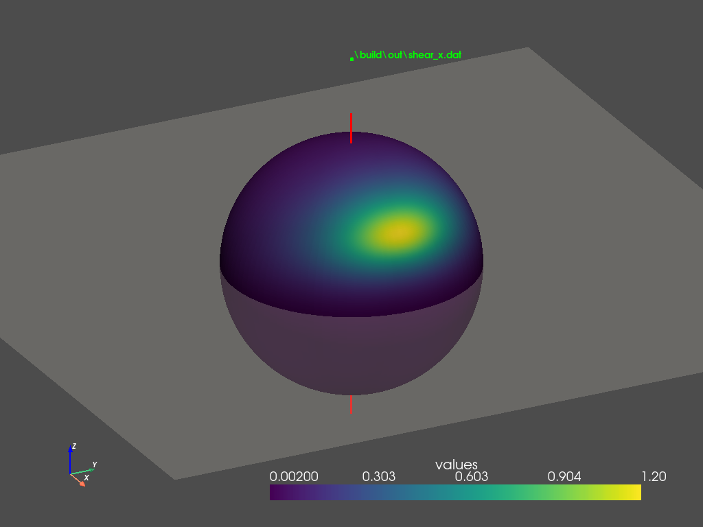
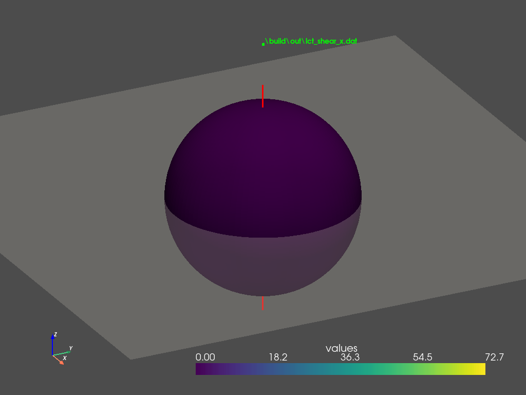
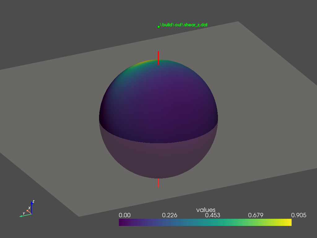
\[\begin{equation} \mathbf{m} = \begin{bmatrix} m_{11} & 0 & 0 \\ 0 & m_{22} & 0 \\ m_{31} & 0 & 1 \end{bmatrix} \label{eq:m-z-shear} \end{equation}\]Shearing along $z$-direction also skews the cosine distribution, as illustrated in Figure 3 (a). By comparing Figure 2 (c) and Figure 3 (c), we can observe that shearing in either direction also produces similar results in the frontal region, where the majority of the distribution lobe lies. This raises the question of why the author chooses to formulate $\mathbf{m}$ in the form of \eqref{eq:m-x-shear} instead of \eqref{eq:m-z-shear}?
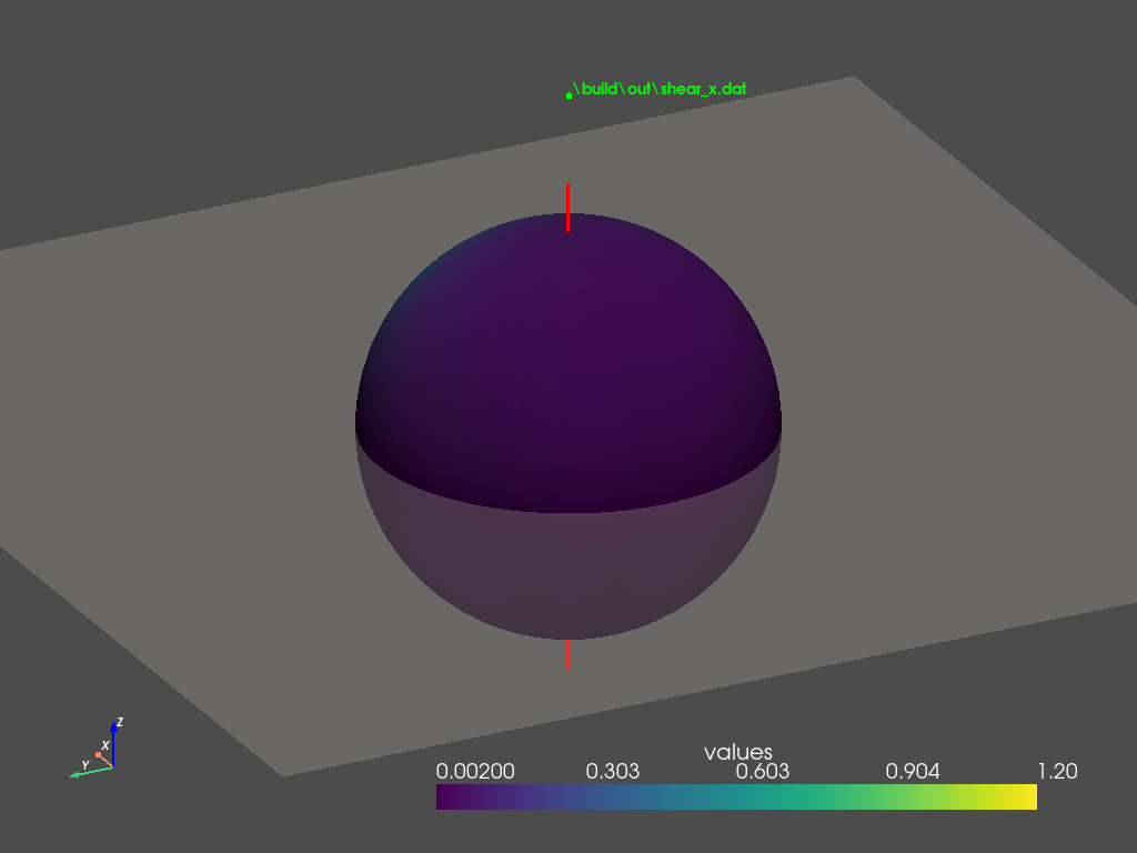
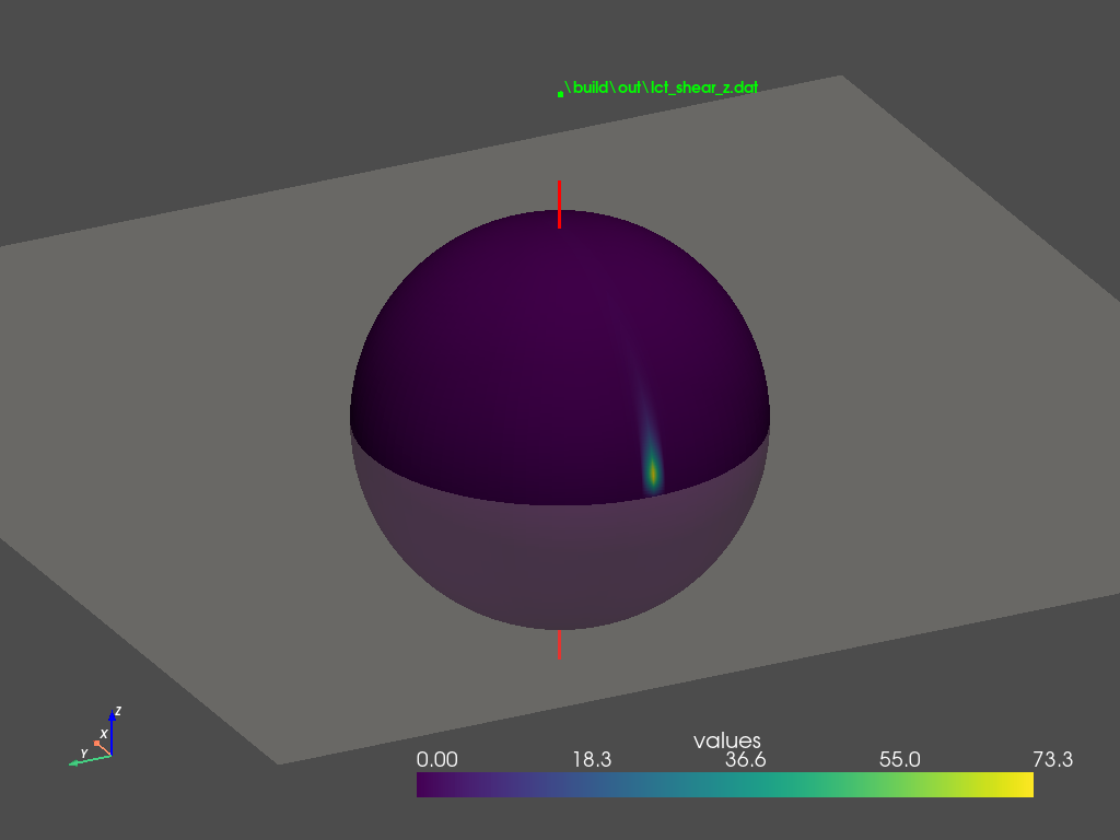
We examine the distributions in the back region, as shown in Figure 2 (d) and Figure 3 (d). $z$-shearing introduces a secondary lobe in the back. This lobe becomes more noticeable for smaller roughness values under grazing angles. In contrast, $x$-shearing does not produce this lobe therefore better approximates GGX BRDFs. This observation explains why the author favors the $x$-direction formulation in \eqref{eq:m-x-shear}.
The secondary lobe problem can be explained by Figure 2 (b) and Figure 3 (b). $x$-shearing effectively ‘shifts’ the cosine lobe towards the front, leaving no energy in the back, whereas $z$-shearing ‘tilts’ the cosine lobe, leaving traces of energy scattered the back region. This residual energy is inherent to $z$-shearing and cannot be removed by rotating the lobe or adjusting the shearing and scaling parameters.


Preconditioning Roughness and Viewing Angle
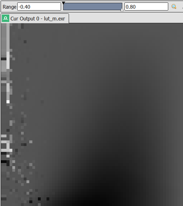
If we fit each $\mathbf{m}$ separately, the parameters become inconsistent. An example is shown in Figure 4 (a), where each shearing factor $m_{13}$ is fitted to its own optimum at each entry. The resulting $\mathbf{m}$ is not necessarily wrong, but a linear filter will behave incorrectly on textures with high-frequency edges.
In the low-roughness region, $m_{13}$ fluctuates erratically between negative and positive values. This happens because for small roughness, BRDF lobes appear as spikes whose shapes are governed mainly by the $x$- and $y$-scaling factors rather than shearing. Owing to the discontinuous nature of Nelder–Mead, the optimizer often finds that the energy difference between the transformed cosine and the target BRDF is small regardless of $m_{13}$, and so it settles on essentially random values.
A reasonably good preconditioning scheme is to use the optimized parameters from an adjacent cell in the lookup texture as the initial guess. Since erratic values appear more often in low-roughness and grazing-angle regions, we start from more ‘tolerant’ regions where roughness is high and the viewing angle is steep, i.e., the top-right corner of the texture. Here, $\mathbf{m}$ is almost an identity matrix, making it a good starting point.
Our goal is to generate parameters for the table entry at the end of the blue arrow in Figure 5. Starting from the top-right corner, we use the optimized $\mathbf{m}$ as the initial guess for the next lower roughness level, moving left until the target roughness is reached (red arrow). We then move downward toward the grazing angles (blue arrow). This way, we cover every viewing-angle/roughness pair in the lookup texture.
A much smoother result obtained through this preconditioning scheme is shown in Figure 4 (b).
